Backprop through time

A recurrent neural network (RNN) reads a sentence one word at a time. At each step it combines the vector for the current word with its hidden state, a short list of numbers that summarizes the words read so far, and it uses the same weights at every step. To train an RNN as a language model on "we sat on the bank of the river", we need to know how each weight should change so that "river" becomes more likely after "we sat on the bank of the". We'll unroll the network into a deep feed-forward network, run backpropagation through it, and then follow the gradient from "river" back to "we" in a network small enough to compute by hand.

Training needs a gradient for every weight

The RNN computes each new state from the vector $\mathbf{x}_t$ of word $t$ and the previous state $\mathbf{h}_{t-1}$:

$$\mathbf{h}_t = \tanh(\mathbf{W}\mathbf{x}_t + \mathbf{U}\mathbf{h}_{t-1} + \mathbf{b})$$

The matrix $\mathbf{W}$ weighs the word, $\mathbf{U}$ weighs the previous state and $\mathbf{b}$ is a bias. The hyperbolic tangent, $\tanh$, squashes each number of the sum into the range from $-1$ to $1$, and the state starts at $\mathbf{h}_0 = \mathbf{0}$. After the seventh word, an output layer turns $\mathbf{h}_7$ into a probability for every word in the vocabulary. With the context $c$ = "we sat on the bank of the", the loss for this prediction is the negative log probability of the correct word:

$$L = -\log P(\text{river} \mid c)$$

Training lowers $L$ by gradient descent. Each weight $\theta$ moves a small step against the derivative of the loss, scaled by a learning rate $\eta$:

$$\theta \leftarrow \theta - \eta \, \frac{\partial L}{\partial \theta}$$

In a feed-forward network, backpropagation computes these derivatives [1]. A forward pass computes the output of every layer. A backward pass then applies the chain rule from the loss down through the layers, and each layer reuses the gradient already computed for the layer above it. An RNN has a loop where a feed-forward network has a stack of layers, so before we can run backpropagation we have to turn the loop into layers.

An unrolled RNN is a deep feed-forward network

We can draw a separate copy of the RNN step for every word. Each copy takes the state from the copy before it and passes its own state to the next, and the loop becomes a chain:

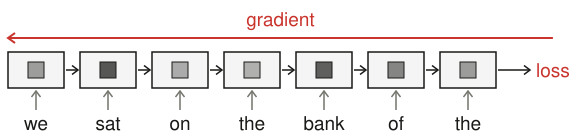
The chain is a feed-forward network with one layer per word: seven layers between "we" and the prediction of "river", and fifty for a sentence of fifty words. Two things set it apart from an ordinary deep network. Every layer reads an input of its own, the vector of its word. And every layer uses the same $\mathbf{W}$, $\mathbf{U}$ and $\mathbf{b}$, where an ordinary network has separate weights in each layer.

Backpropagation through time

Running backpropagation on the unrolled chain is called backpropagation through time (BPTT) [2]. The forward pass runs the RNN over the sentence and keeps every state, $\mathbf{h}_1$ to $\mathbf{h}_7$, along with the loss. The backward pass starts from the gradient of the loss with respect to the last state, $\partial L / \partial \mathbf{h}_7$, and moves one step to the left at a time:

$$\frac{\partial L}{\partial \mathbf{h}_{t-1}} = \frac{\partial L}{\partial \mathbf{h}_t} \, \frac{\partial \mathbf{h}_t}{\partial \mathbf{h}_{t-1}}$$

Each step back multiplies the gradient by the derivative of one state with respect to the state before it. When the network predicts a word at every step, as a language model does, each step also adds the gradient of its own loss before passing the sum further back.

The derivative at each step depends on that step's state, so the backward pass needs every state the forward pass computed, and memory grows with the length of the text. On long texts a common compromise is truncated BPTT: the backward pass stops after a fixed number of steps, while the forward pass keeps carrying the state forward.

Shared weights add up their gradients

Because $\mathbf{U}$ acts at all seven steps, the loss depends on it seven times. We can compute the gradient as if every step had its own copy $\mathbf{U}_{(t)}$, exactly as backpropagation would for a deep network with separate layers, and then add the gradients of the copies:

$$\frac{\partial L}{\partial \mathbf{U}} = \sum_{t=1}^{7} \frac{\partial L}{\partial \mathbf{U}_{(t)}}$$

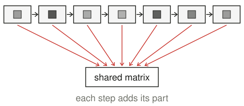
The gradients of $\mathbf{W}$ and $\mathbf{b}$ are sums over the steps in the same way. One update then changes the single shared matrix, so the copies stay identical. The part for step $t$ is built from the gradient that reached that step, $\partial L / \partial \mathbf{h}_t$. For $\mathbf{W}$, the part for step 1 is where "we" enters the update, and it can only be as large as the gradient that made it back from $\mathbf{h}_7$ to $\mathbf{h}_1$.

Each step back multiplies by one factor

To see how much gradient reaches the early steps, we can shrink the network until the state and each word's vector are single numbers. With weights $w$ and $u$ and no bias, the step is

$$h_t = \tanh(w\,x_t + u\,h_{t-1})$$

The derivative of $\tanh(z)$ is $1 - \tanh^2(z)$, so one step back multiplies the gradient by

$$\frac{\partial h_t}{\partial h_{t-1}} = u\,(1 - h_t^2)$$

The factor is the recurrent weight times the slope of $\tanh$ at that step. The slope is $1$ when the state is $0$ and falls toward $0$ as the state nears $-1$ or $1$. Going from $h_7$ back to $h_1$ takes six steps, so the gradient picks up six factors:

$$\frac{\partial h_7}{\partial h_1} = \prod_{t=2}^{7} u\,(1 - h_t^2)$$

Following the gradient from "river" back to "we"

Take $w = 1$ and $u = 0.6$, and give each word one number:

The first state depends only on "we", and the second adds "sat" to what the first carried forward:

$$h_1 = \tanh(-0.2) = -0.20$$ $${h_2 = \tanh(0.6 + 0.6 \cdot (-0.20))} = \tanh(0.48) = 0.45$$

Continuing through "on the bank of the" gives the seven states in the boxes below. The factor between $h_1$ and $h_2$ is $0.6\,(1 - 0.45^2) = 0.48$, and the red numbers are the factors for every step:

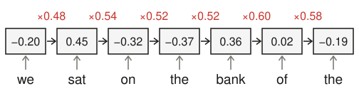
The states stay well inside the range of $\tanh$, so its slope stays close to $1$ and every factor lands just under $u = 0.6$. Multiplying the six factors gives the gradient that reaches $h_1$:

$$\frac{\partial h_7}{\partial h_1} = 0.48 \cdot 0.54 \cdot 0.52 \cdot 0.52 \cdot 0.60 \cdot 0.58 \approx 0.024$$

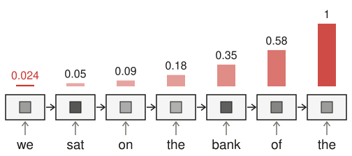
Every step back roughly halves the gradient. After one step it is $0.58$ of what it was at $h_7$, after three steps $0.18$, and by the time it reaches the state after "we", $0.024$:

Vanishing and exploding gradients

Nothing in this calculation is special to seven words. The gradient that travels $k$ steps back is a product of $k$ factors, so it changes exponentially with the distance. If every factor were $0.5$ or $1.5$:

A gradient that shrinks toward zero over many steps is a vanishing gradient, and one that grows without bound is an exploding gradient. A 1994 analysis showed that gradient descent has an increasingly hard time learning a dependency as the number of steps it spans grows [3].

With vector states, each factor is a matrix, the derivative $\partial \mathbf{h}_t / \partial \mathbf{h}_{t-1}$. It multiplies $\mathbf{U}$ by the slope of $\tanh$ for each number of the state, and those slopes are at most $1$. If the largest eigenvalue of $\mathbf{U}$ is smaller than $1$ in absolute value, the long-range parts of the gradient vanish, and they can explode only if it is larger than $1$ [4]. Weights that start small fall in the first case. The states also push toward it: whenever a number of the state nears $-1$ or $1$, its slope, and with it the factor, drops toward $0$.

Clipping caps exploding gradients

An exploding gradient is the easier failure to see. One enormous gradient can throw the weights far from where training had brought them. A simple fix is gradient norm clipping [4]. Before each update, if the length of the gradient $\mathbf{g}$ exceeds a threshold $\tau$, we scale it back to length $\tau$:

$$\text{if } \lVert \mathbf{g} \rVert > \tau: \qquad \mathbf{g} \leftarrow \tau \, \frac{\mathbf{g}}{\lVert \mathbf{g} \rVert}$$

For $\mathbf{g} = (3,\ 4)$ the length is $5$. With $\tau = 1$, clipping gives $(0.6,\ 0.8)$, which points the same way:

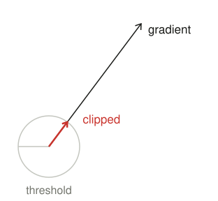
The update keeps its direction and takes a bounded step. The 2013 paper that proposed this rule built on an earlier version from work on RNN language models, which clipped each number of the gradient separately. Its authors suggest choosing $\tau$ by looking at the average length of the gradient over many updates, and report that training is not very sensitive to the exact value.

Early words stop influencing learning

Clipping only shortens a gradient that is too long. A vanished gradient is too short, so there is nothing to clip, and scaling the whole gradient up would not change how little of it comes from the early steps. In our network the gradient from "river" reaches the state after "we" at $0.024$ of its size at the last step. The parts of the update that come from the early steps are correspondingly small, and the sum is dominated by the last few words. Training learns how "bank of the" predicts "river" and gets almost no signal about "we sat on", the words that make this a bank someone sits beside. Truncated BPTT cuts the early words off at a fixed distance; vanishing gradients fade them out over a few steps even when the backward pass runs the full length of the sentence.

References

1. Rumelhart, D. E., Hinton, G. E., & Williams, R. J. (1986). Learning representations by back-propagating errors. Nature 323. doi:10.1038/323533a0 ↩
2. Werbos, P. J. (1990). Backpropagation through time: what it does and how to do it. Proceedings of the IEEE 78(10). doi:10.1109/5.58337 ↩
3. Bengio, Y., Simard, P., & Frasconi, P. (1994). Learning long-term dependencies with gradient descent is difficult. IEEE Transactions on Neural Networks 5(2). doi:10.1109/72.279181 ↩
4. Pascanu, R., Mikolov, T., & Bengio, Y. (2013). On the difficulty of training recurrent neural networks. Proceedings of the 30th International Conference on Machine Learning. proceedings.mlr.press ↩