The co-occurrence matrix: words described by their neighbors

A model that counts words treats each one as a separate symbol. Counts for "bank" tell it nothing about "shore", even though the two words can stand in the same place in a sentence. To let similar words share what is known about them, we need a description of each word that can be compared with the descriptions of other words.

We'll build that description from the words that appear around each word. Working through the sentence "we sat on the bank of the river", we'll count neighbors into a matrix, compare its rows, reweight the counts and compress the result.

Words are known by their neighbors

Words that occur in similar contexts tend to have similar meanings. This is the distributional hypothesis: Harris argued that differences in meaning correlate with differences in the environments where words appear [1], and Firth summarized the idea as "You shall know a word by the company it keeps" [2].

Consider the gap in "we sat on the ___ of the river". Both "bank" and "shore" fit, and the words around the gap are what allow either. If we record, for every word, which words tend to surround it, then "bank" and "shore" should end up with similar records.

Count the words in a window

A context window covers the words up to a fixed distance on each side of a word. With two positions on each side, the window around "bank" holds "on", "the", "of" and "the":

Each word inside the window adds 1 to the count for that pair of words. "The" appears twice in the window, so the pair (bank, the) gets a count of 2, while "on" and "of" get 1 each.

Every word gets a row

We move the window to every position in the sentence and add up the counts. The result is a co-occurrence matrix: one row for each word, one column for each context word, and in each cell the number of times the context word appeared within two positions of the row's word.

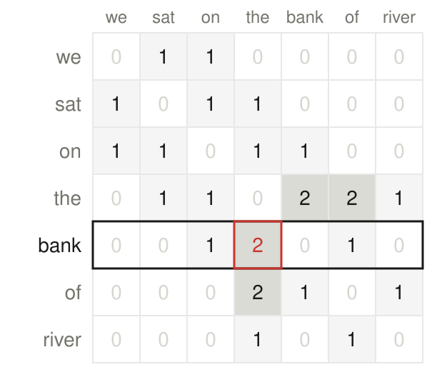
The matrix is symmetric, because "bank" being within two words of "the" is the same event as "the" being within two words of "bank". Over a large corpus the same procedure runs across millions of sentences, and each row summarizes how its word is used.

Compare rows by their angle

Each row is a vector of counts, so comparing two words means comparing two vectors. Frequent words have large counts in every column, which makes their vectors long. To compare directions rather than lengths, we use cosine similarity, the cosine of the angle between two vectors:

$$\cos(\mathbf{a},\mathbf{b}) = \frac{\mathbf{a}\cdot\mathbf{b}}{\lVert\mathbf{a}\rVert\,\lVert\mathbf{b}\rVert}$$

Counts are never negative, so the cosine ranges from 0, for words with no context in common, to 1, for words whose counts are proportional.

To see "bank" and "shore" side by side, we add a second sentence, "we sat on the shore of the lake", and count both sentences together. These are the columns where "bank", "shore" and "river" have non-zero counts:

	on	the	of
bank	1	2	1
shore	1	2	1
river	0	1	1

"Shore" has exactly the window counts of "bank", so their cosine is 1. "River" shares only "the" and "of" with "bank":

$${\cos(\text{bank},\text{river})} = {\frac{1\cdot 0+2\cdot 1+1\cdot 1}{\sqrt{6}\,\sqrt{2}}} \approx 0.87$$

That score is high for two words that can't replace each other. Two of the 3 in the numerator come from "the", the largest count in the "bank" row.

Weight the surprising neighbors

"The" appears near almost every noun, so a high count with "the" says little about any particular word. What matters is whether two words occur together more often than their separate frequencies would predict. Pointwise mutual information (PMI) measures exactly that, comparing the probability of seeing the pair with the probability expected if the two words were independent [3]:

$$\text{PMI}(w,c) = \log_2\frac{P(w,c)}{P(w)\,P(c)}$$

Here $P(w,c)$ is the pair's count divided by the total of all counts, and $P(w)$ and $P(c)$ are the row and column totals divided by the same number. A negative PMI means two words meet less often than chance, and with limited text those estimates are unreliable, so we use positive PMI and replace negative values with 0:

$$\text{PPMI}(w,c) = \max\bigl(\text{PMI}(w,c),\,0\bigr)$$

The two sentences contain 52 counts in total. "River" meets "of" once and "the" once, but "the" fills 14 of the 52 context slots and "of" fills 8:

The two raw counts were equal, and PPMI gives the rarer context almost twice the weight. Recomputing every cell with PPMI lowers $\cos(\text{bank},\text{river})$ from 0.87 to 0.78, while "bank" and "shore" keep a cosine of 1. Down-weighting contexts that appear everywhere is the same move tf-idf makes for words that appear in every document.

The window size changes the neighbors

The window width decides what the counts capture:

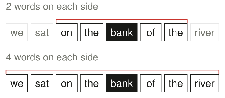
With two words on each side, "bank" is described by "on the" and "of the", words that frame the grammatical slot it fills. With four, "we", "sat" and "river" join in, words that describe the scene. Small windows therefore group words that can replace each other, like "bank" and "shore"; large windows group words that appear in the same topics, like "bank" and "river".

The matrix is huge and mostly zeros

Our matrix has 7 rows. A realistic vocabulary of 100,000 words gives one row and one column for every word:

$$100{,}000^2 = 10{,}000{,}000{,}000 \text{ cells}$$

Most pairs of words never appear near each other, so nearly all of those cells are 0. Even the matrix from our single sentence has 27 zeros among its 49 cells. Vectors that are mostly zeros are called sparse. Each word is described by 100,000 numbers, and two rare words may share no non-zero column even when they mean nearly the same thing.

Compress the counts

Truncated singular value decomposition (SVD) approximates the matrix $\mathbf{X}$ with a product of three much smaller matrices:

$$\mathbf{X} \approx \mathbf{U}_k\,\boldsymbol{\Sigma}_k\,\mathbf{V}_k^{\top}$$

$\boldsymbol{\Sigma}_k$ holds the $k$ largest singular values, the strengths of the $k$ directions along which the rows vary most, and each row of $\mathbf{U}_k\boldsymbol{\Sigma}_k$ is a word's vector in those directions. With $k$ in the low hundreds, every word gets a short, dense vector. Words that never shared a context directly can still end up close, because their neighbors share contexts. Latent semantic analysis applied this decomposition to word counts across documents [4].

Compression doesn't change where the numbers come from. The full matrix still has to be counted before it can be decomposed, and the dense vectors are still a summary of those counts. No step adjusts them to make predicting the next word, or any other task, work better.

References

1. Harris, Z. S. (1954). Distributional Structure. Word 10(2-3). doi:10.1080/00437956.1954.11659520 ↩
2. Firth, J. R. (1957). A Synopsis of Linguistic Theory, 1930-1955. Studies in Linguistic Analysis, Basil Blackwell. archive.org ↩
3. Church, K. W., & Hanks, P. (1990). Word Association Norms, Mutual Information, and Lexicography. Computational Linguistics 16(1). aclanthology.org ↩
4. Deerwester, S., et al. (1990). Indexing by Latent Semantic Analysis. Journal of the American Society for Information Science 41(6). doi:10.1002/(SICI)1097-4571(199009)41:6<391::AID-ASI1>3.0.CO;2-9 ↩