Feed-forward neural networks

A language model built from counts gives each word a fixed set of numbers, and nothing in those numbers changes when a prediction goes wrong. To learn from mistakes, we need a model whose parameters move to reduce error. A feed-forward neural network is that kind of model: layers of simple units, each a weighted sum followed by a nonlinearity, trained by sending the error backward through the layers. We'll build one from a single unit and use it to compute XOR, a function no single weighted sum can represent.

One unit: weighted sum, then activation

A single unit takes a vector of inputs $\mathbf{x}$, multiplies each coordinate by a weight, and adds a bias. The result is the pre-activation:

$$z = \mathbf{w}\cdot\mathbf{x} + b = w_1 x_1 + w_2 x_2 + b$$

An activation function $f$ turns $z$ into the unit's output $a = f(z)$. Early linear classifiers used a hard threshold (the step function) as $f$, which yields the perceptron [1]. The step is not differentiable, so gradient methods cannot follow it. The sigmoid (logistic) function is a smooth alternative that maps any real $z$ into $(0,1)$:

$$\sigma(z) = \frac{1}{1+e^{-z}}$$

As $z \to +\infty$, $\sigma(z)$ approaches 1; as $z \to -\infty$, it approaches 0. Other common choices include $\tanh$ and the rectified linear unit $\operatorname{ReLU}(z)=\max(z,0)$. Without some nonlinearity, stacking units collapses: a composition of linear maps is still one linear map, so the whole stack could be replaced by a single weighted sum.

XOR: a function no line can separate

Consider two binary inputs and the XOR function: the output is 1 when exactly one input is 1, and 0 otherwise.

$x_1$	$x_2$	XOR
0	0	0
0	1	1
1	0	1
1	1	0

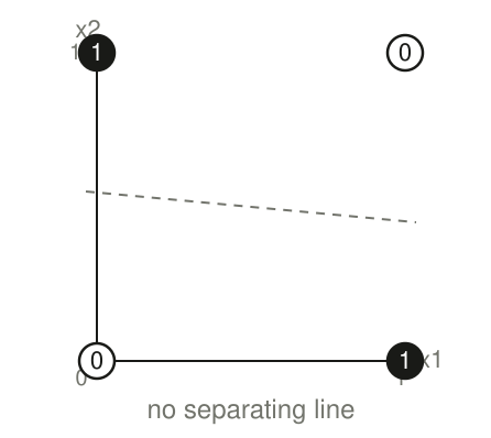
Plotted in the plane, the two positive points sit on opposite corners of the unit square, and the two negatives on the other pair. No straight line places both positives on one side and both negatives on the other. A single unit that computes $f(\mathbf{w}\cdot\mathbf{x}+b)$ with a monotone $f$ draws exactly one such boundary, so it cannot represent XOR [2].

Layers compose simple units

A feed-forward network stacks units into layers. The first hidden layer receives the inputs; each later layer receives the previous layer's activations; the output layer produces the prediction. There are no loops: information flows in one direction.

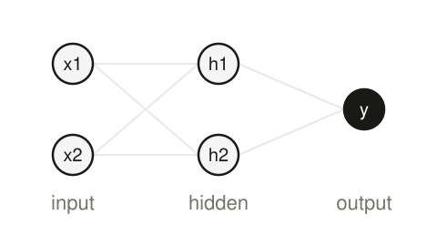
With $n$ inputs, a hidden layer of $m$ units and $K$ output classes, the network computes

$$\mathbf{h} = f(\mathbf{W}\mathbf{x} + \mathbf{b})$$ $$\mathbf{z} = \mathbf{V}\mathbf{h} + \mathbf{b}'$$

where $\mathbf{W}$ is $m \times n$ and $\mathbf{V}$ is $K \times m$. The hidden layer re-describes $\mathbf{x}$ in new coordinates, and the output layer scores each class in those coordinates. With a nonlinear $f$ the whole map is nonlinear, and one hidden layer with enough units can approximate any continuous function on a bounded region to any accuracy [3].

Two hidden units are enough for XOR. We'll use the step function, which outputs 1 for a positive input and 0 otherwise, to keep the arithmetic exact. The first unit fires when at least one input is on, the second only when both are on, and the output subtracts the second from the first:

$$h_1 = \operatorname{step}(x_1 + x_2 - 0.5)$$ $$h_2 = \operatorname{step}(x_1 + x_2 - 1.5)$$ $$y = \operatorname{step}(h_1 - h_2 - 0.5)$$

For $(0,1)$ we get $h_1 = 1$ and $h_2 = 0$, so $y = 1$. For $(1,1)$ both hidden units fire, the output's input is $-0.5$, and $y = 0$. For $(0,0)$ neither fires and $y = 0$. In the hidden coordinates $(h_1, h_2)$ the inputs land on three points, $(0,0)$, $(1,0)$ and $(1,1)$, and a single line separates $(1,0)$ from the other two. A sigmoid with large weights behaves almost like this step, and because it is differentiable, gradient descent can find such weights from the four examples.

Softmax turns scores into probabilities

Many language tasks are multi-class: each output coordinate is one class. Softmax converts a vector of scores $\mathbf{z}$ into a probability distribution over the classes:

$$P(y=k \mid \mathbf{x}) = \frac{e^{z_k}}{\sum_j e^{z_j}}$$

Each probability is positive, and the values sum to 1. The class with the largest score receives the largest probability.

Loss measures how wrong the prediction is

Given a training example $(\mathbf{x}, y^*)$ with correct class $y^*$, negative log-likelihood (cross-entropy) charges the model for assigning low probability to $y^*$:

$$L = -\log P(y^* \mid \mathbf{x})$$

When the model puts probability $1$ on the correct class, $L=0$. When it puts probability $0.1$ on it, $L = -\log 0.1 \approx 2.3$. Averaging $L$ over the training set gives the empirical risk we minimize.

Backpropagation sends error to every weight

The network's weights start random. Gradient descent updates each weight a small step opposite the derivative of the loss:

$$w \leftarrow w - \eta \frac{\partial L}{\partial w}$$

where $\eta$ is the learning rate. Softmax and sigmoid are differentiable, so the chain rule gives $\partial L/\partial w$ for every weight once we know how $L$ depends on the outputs.

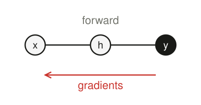
Backpropagation organizes that calculation [4]. A forward pass computes every pre-activation and activation from the inputs to the loss. A backward pass starts from $\partial L/\partial \mathbf{y}$ and applies the chain rule through each layer in reverse, yielding the gradient for every weight matrix and bias.

After many updates the weights encode a nonlinear decision rule fitted to the training data. Unlike a co-occurrence matrix of fixed counts, these numbers move when the loss says the prediction was wrong.

Words still wait outside the network

A feed-forward network learns a map from vectors of real numbers to probabilities. Language arrives as discrete words, as in "we sat on the bank of the river". Until each word has an input vector, and the output layer has one score per word in the vocabulary, the network has nothing to read and nothing to predict.

References

1. Rosenblatt, F. (1958). The Perceptron. Psychological Review 65(6). doi:10.1037/h0042519 ↩
2. Minsky, M., & Papert, S. (1969). Perceptrons. MIT Press. ↩
3. Hornik, K., Stinchcombe, M., & White, H. (1989). Multilayer feedforward networks are universal approximators. Neural Networks 2(5). doi:10.1016/0893-6080(89)90020-8 ↩
4. Rumelhart, D. E., Hinton, G. E., & Williams, R. J. (1986). Learning representations by back-propagating errors. Nature 323. doi:10.1038/323533a0 ↩