How do hidden Markov models work?

A language model predicts a word $w$ from its context $c$, the words that come before it. Counting which words follow which gives one estimate of $P(w \mid c)$, but those counts ignore a pattern every reader of English relies on: words fall into grammatical classes, and the classes follow each other in predictable ways. After "the", we expect a noun or an adjective before we know which word it will be.

We'll build a model of that hidden structure, a hidden Markov model (HMM). We'll use it to label each word in a sentence with its grammatical class, then use the same model to predict the next word.

Words carry hidden tags

A part-of-speech tag marks the grammatical role a word plays: noun, verb, determiner, preposition and so on. The Universal Dependencies project defines 17 tags for annotating text consistently across languages [1]. Here is a sentence with its tags:

PRONwe

VERBsat

ADPon

DETthe

NOUNbank

ADPof

DETthe

NOUNriver

PRON marks a pronoun, DET a determiner such as "the", and ADP an adposition, which in English is a preposition such as "on" or "of". Assigning one tag to every word is part-of-speech tagging. It is a sequence labeling task: the input is a sequence of words, and the output is a sequence of tags of the same length.

Tagging would be simple if every word had only one possible tag. "Bank" is a noun in our sentence and a verb in "we bank on it":

DETthe

NOUNbank

ADPof

DETthe

NOUNriver

PRONwe

VERBbank

ADPon

PRONit

The word alone doesn't settle its tag; the neighboring tags do. After the determiner "the", a noun is far more likely than a verb, while a pronoun such as "we" is often followed by a verb. A tagger has to weigh how well each tag fits the word against how well it fits the tags around it.

A model that generates tags, then words

An HMM describes how a tagged sentence could have been produced, in two steps. First it chooses a sequence of tags, each depending only on the tag before it. Then each tag produces a word.

START

→

DET↓the

→

NOUN↓bank

→

ADP↓of

→

DET↓the

→

NOUN↓river

The probability of moving from one tag to the next, $P(t_i \mid t_{i-1})$, is a transition probability. The tag sequence is a bigram model over tags: the Markov assumption that a bigram language model makes about words, applied to tags instead. A special START tag $t_0$ begins every sentence, so the first tag has a predecessor too.

The probability that a tag produces a particular word, $P(w_i \mid t_i)$, is an emission probability. In the notation $P(w \mid c)$, the context of each word is now its tag. We observe the words but not the tags, which is what makes this Markov model hidden [2].

Multiplying a transition and an emission for each word gives the probability of the words together with one particular tag sequence:

$${P(w_1,\ldots,w_n,\;t_1,\ldots,t_n)} = {\prod_{i=1}^{n} P(t_i\mid t_{i-1})\,P(w_i\mid t_i)}$$

Count transitions and emissions

Given text in which people have tagged every word, we can estimate both kinds of probability by counting. A transition probability divides the number of times one tag follows another by the number of times the first tag appears:

$$\widehat{P}(t_i\mid t_{i-1}) = \frac{\operatorname{count}(t_{i-1},t_i)}{\operatorname{count}(t_{i-1})}$$

An emission probability divides the number of times a word appears with a tag by the number of times that tag appears:

$$\widehat{P}(w_i\mid t_i) = \frac{\operatorname{count}(t_i,w_i)}{\operatorname{count}(t_i)}$$

Suppose 60% of the determiners in our tagged text are followed by a noun and 2% by a verb, and "bank" makes up 0.2% of the nouns and 0.05% of the verbs:

We can now compare the two readings of "bank" after "the". Each reading contributes one transition from DET and one emission of "bank":

The noun reading is 120 times more probable. The emissions alone favor the noun by a factor of 4; the transition from DET contributes the other factor of 30. Most of the decision comes from the neighboring tag.

Find the best tag sequence

Tagging a sentence means finding its most probable tag sequence. The words are fixed, so this is the tag sequence with the highest joint probability.

The direct approach scores every tag sequence. If any of the 17 tags can appear at each position, our eight-word sentence has

$$17^8 = 6{,}975{,}757{,}441$$

possible sequences, and each additional word multiplies the number by 17. We can draw the choices as a trellis, a grid with one column per word and one row per tag, where every left-to-right path is one tag sequence.

The Viterbi algorithm finds the best path without enumerating them. Andrew Viterbi introduced it in 1967 to decode error-correcting codes [3], and HMMs have the same structure. Suppose two partial paths both end with NOUN at "bank". Everything after "bank" depends only on that NOUN tag, not on how the path reached it, so the lower-scoring path can never be part of the best complete sequence. For each word and each tag, we keep only the best path that ends there.

We write $v_i(t)$ for the probability of that path: the highest probability of the first $i$ words together with any tag sequence ending in tag $t$. Each column of the trellis follows from the previous one:

$$v_i(t) = {\max_{t'}\; v_{i-1}(t')\,P(t\mid t')\,P(w_i\mid t)}$$

The sweep starts from $v_0(\text{START}) = 1$. Alongside each $v_i(t)$, we store the previous tag $t'$ that gave the maximum.

At "bank", the fifth word, the best paths into both readings come through DET for "the":

$$\begin{aligned} v_5(\text{NOUN}) &= v_4(\text{DET})\times0.6\times0.002 \\ v_5(\text{VERB}) &= v_4(\text{DET})\times0.02\times0.0005 \end{aligned}$$

Both readings can continue to ADP for "of". The algorithm compares $v_5(\text{NOUN})\,P(\text{ADP}\mid\text{NOUN})$ with $v_5(\text{VERB})\,P(\text{ADP}\mid\text{VERB})$ and keeps the larger. The noun path starts 120 times ahead, and prepositions follow nouns about as readily as verbs, so the path through NOUN survives. After the last word, we take the tag with the highest $v_8$ and follow the stored choices back to the start. Here is that trace, with five of the 17 tags shown:

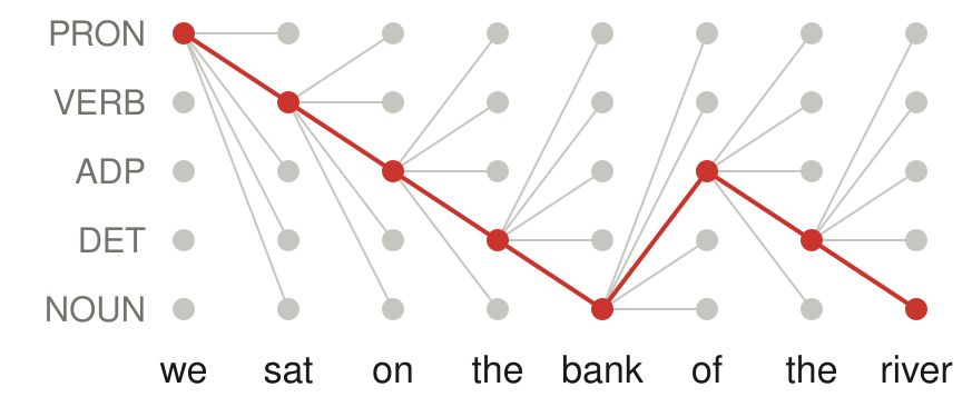
Each step considers 17 tags for the current word and 17 previous tags, so tagging our sentence takes about $8\times17\times17 = 2{,}312$ steps instead of nearly seven billion. The work grows in proportion to sentence length. HMM taggers built this way, with probabilities counted from tagged text, became the standard approach to part-of-speech tagging in the late 1980s [4].

Sum the paths to predict words

The Viterbi algorithm keeps the single best path. If we add up the probabilities of all paths instead, we get the probability of the words themselves, whatever their tags:

$${P(w_1,\ldots,w_n)} = {\sum_{t_1,\ldots,t_n} P(w_1,\ldots,w_n,\;t_1,\ldots,t_n)}$$

The forward algorithm computes this sum in the same left-to-right sweep, with a sum in place of the maximum [2]:

$$\alpha_i(t) = {\sum_{t'} \alpha_{i-1}(t')\,P(t\mid t')\,P(w_i\mid t)}$$

Here $\alpha_i(t)$ is the total probability of the first $i$ words over all tag paths that end in $t$, and adding up $\alpha_8(t)$ over the tags gives the probability of the whole sentence. An HMM therefore assigns probabilities to sentences, like any language model, and it can predict the next word. With $c$ the words so far and $t$ the tag of the next word:

$$P(w\mid c) = \sum_{t} P(t\mid c)\,P(w\mid t)$$

The tag probabilities $P(t \mid c)$ come from the forward values for the words so far, passed through one more transition. After "we sat on the bank of the", most of the probability goes to NOUN and much of the rest to ADJ. Every earlier word contributes to these values, so the context is not cut off at a fixed number of words as it is in an n-gram model.

That context reaches the next word through a narrow channel: one probability for each of the 17 tags. Once the model expects a noun after "bank of the", it ranks the candidates by $P(w \mid \text{NOUN})$, regardless of which words came before. "Year" appears as a noun far more often than "river", so the model prefers "we sat on the bank of the year". Tags let rare words share statistics with the rest of their class, but the classes are designed by linguists, the counts require text tagged by hand, and within a class each word's probability is estimated separately, so nothing the model learns about "river" helps it with "stream".

References

1. Nivre, J., et al. (2020). Universal Dependencies v2: An Evergrowing Multilingual Treebank Collection. Proceedings of LREC 2020. aclanthology.org ↩
2. Rabiner, L. R. (1989). A Tutorial on Hidden Markov Models and Selected Applications in Speech Recognition. Proceedings of the IEEE 77(2). doi:10.1109/5.18626 ↩
3. Viterbi, A. J. (1967). Error Bounds for Convolutional Codes and an Asymptotically Optimum Decoding Algorithm. IEEE Transactions on Information Theory 13(2). doi:10.1109/TIT.1967.1054010 ↩
4. Church, K. W. (1988). A Stochastic Parts Program and Noun Phrase Parser for Unrestricted Text. Proceedings of the Second Conference on Applied Natural Language Processing. aclanthology.org ↩