Neural language models

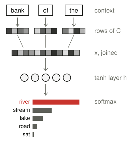
A language model predicts the next word $w$ from its context $c$, the words that came before it. Counting models estimate $P(w \mid c)$ by looking up how often $w$ followed that exact context, and every word is a separate symbol with nothing in common with any other word. A neural language model replaces the count table with a feed-forward network that reads each context word as a vector of learned numbers. We'll follow one prediction through such a network, the word after "bank of the" in the sentence "we sat on the bank of the river", and see why words used in similar ways end up sharing what the model learns.

Counts don't transfer between contexts

An n-gram model takes the context to be the last $n-1$ words. With three context words, it estimates the probability of "river" by counting:

$$P(\text{river} \mid \text{bank, of, the}) = \frac{\text{count}(\text{bank of the river})}{\text{count}(\text{bank of the})}$$

Each exact context gets its own row of counts. If the training text contains "bank of the river" but never "shore of the river", the model has no count for the second context, even though "shore" and "bank" are used in nearly the same way. Smoothing and backoff give the unseen context some probability by falling back to shorter contexts, such as "of the", which throws away the most informative word.

The space of contexts is also far too large to fill. With a vocabulary of 100,000 words there are $100{,}000^{10} = 10^{50}$ possible sequences of ten words [1], so almost every long context in new text is one the training data never contained.

Each word becomes a learned vector

The neural language model of Bengio and colleagues [1] gives every word in the vocabulary $V$ a vector of $m$ real numbers, its word embedding. The embeddings are the rows of a matrix $\mathbf{C}$ with $|V|$ rows and $m$ columns, and reading a word means looking up its row $C(w)$. If $\mathbf{o}_w$ is the one-hot vector with a 1 in the position of word $w$, the lookup is an ordinary matrix product:

$$C(w) = \mathbf{o}_w^{\top}\,\mathbf{C}$$

So the embedding table is simply the first layer of the network, a linear layer whose weights are the word vectors. The rows start out random. Nothing about "bank" is written in by hand; its numbers come only from training. Representing a concept as a pattern over many learned features, rather than as one symbol, is called a distributed representation [2].

The context becomes one input vector

For the context $c = (\text{bank}, \text{of}, \text{the})$ we look up three rows and place them side by side:

$$\mathbf{x} = \big[\,C(\text{bank});\ C(\text{of});\ C(\text{the})\,\big]$$

With $m$ numbers per word, $\mathbf{x}$ has $3m$ numbers. Each position keeps its own slot, so the network still knows which word came first. The same matrix $\mathbf{C}$ supplies every position, so "the" has the same vector wherever it appears.

A hidden layer combines the context

The input vector goes through one hidden layer with the hyperbolic tangent as its nonlinearity:

$$\mathbf{h} = \tanh(\mathbf{H}\mathbf{x} + \mathbf{d})$$

$\tanh$ has the same S shape as the sigmoid but outputs values between $-1$ and $1$. Because $\mathbf{H}$ sees all three word vectors at once, a hidden unit can respond to combinations, such as a noun followed by "of the", that no single word signals on its own.

Softmax scores every word in the vocabulary

The output layer produces one score per vocabulary word, and softmax turns the scores into the next-word distribution:

$$\mathbf{y} = \mathbf{U}\mathbf{h} + \mathbf{b}$$ $$P(w_t = i \mid c) = \frac{e^{y_i}}{\sum_{j} e^{y_j}}$$

$\mathbf{U}$ has $|V|$ rows, so $\mathbf{y}$ has $|V|$ entries. To see the arithmetic, we can shrink the vocabulary to five words. With scores $2.1$ for river, $1.2$ for stream, $0.6$ for lake, $-0.2$ for road and $-1.5$ for sat, softmax gives river $0.569$, stream $0.231$, lake $0.127$, road $0.057$ and sat $0.016$. The five probabilities sum to 1, and the ordering of the scores is kept.

Training moves the embeddings too

The model is trained on running text. At each position the correct next word is known, and the loss is its negative log-probability. For our example, where "river" received $0.569$:

$$L = -\log P(\text{river} \mid \text{bank, of, the}) = -\log 0.569 \approx 0.56$$

Backpropagation sends the gradient of $L$ through $\mathbf{U}$ and $\mathbf{H}$ as in any feed-forward network, and then one step further, into $\mathbf{x}$. Since $\mathbf{x}$ is just three rows of $\mathbf{C}$, those three rows get updated as well. The embeddings, the hidden layer and the output layer are all fitted together to make the training text likely.

Similar words end up with similar vectors

Suppose "bank" and "shore" both show up before words like "of the river" and "of the lake" in the training text. Every time, the gradient nudges each word's vector toward values that make those same continuations likely, so the two vectors drift toward each other. Words that appear in similar contexts end up with similar embeddings.

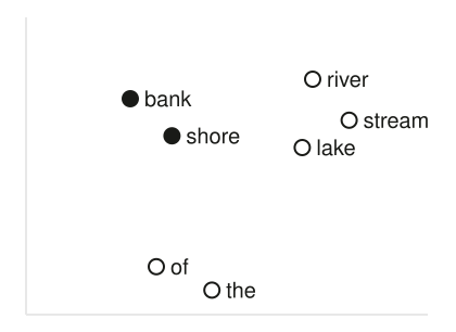
Now take the context "shore of the", which may never have appeared in training. Its input vector is close to the one for "bank of the", so the hidden layer responds in nearly the same way and "river" again gets a high probability. The count table had no row for this context. The network generalizes from one context to another through the similarity of their word vectors.

The network also needs far fewer numbers than the space of contexts. Its parameters are the embeddings, the hidden weights and biases, and the output weights and biases:

$${|V|\,m + h\,(n-1)\,m + h} \;+\; {|V|\,h + |V|}$$

With $|V| = 10{,}000$, $m = 100$, three context words and $h = 200$ hidden units, that is $3{,}070{,}200$ parameters. A table of 4-grams over the same vocabulary has $10{,}000^4 = 10^{16}$ possible entries. Adding a fourth context word adds $m\,h = 20{,}000$ weights to $\mathbf{H}$, rather than multiplying the number of contexts by $10{,}000$.

Better predictions at a high cost

The 2003 experiments measured perplexity, the geometric mean of $1/P(w \mid c)$ over the words of the test text, where lower means the model was less surprised. On the Brown corpus, about 1.2 million words of varied English, the best n-gram model scored 312. That model was class-based: it grouped words into 500 classes and shared counts within each class [3], an earlier way of letting similar words pool statistics. The networks on their own reached 268, and averaging a network's probabilities with a simple trigram model's brought the test perplexity down to 252. On the larger AP News corpus, about 14 million words, the network's advantage was about 8%. On Brown, extending the context from two words to four helped the network but not the n-gram models.

The cost sits in the output layer. Every prediction computes a score for every word in the vocabulary before softmax can normalize, and every training example sends gradients back through all of those scores. On AP News, five passes over the data took about three weeks on 40 CPUs [1].

The window is still fixed

The network reads exactly $n-1$ words. Predicting "river" from "bank of the" ignores "we sat on", the words that tell us this is a bank someone can sit on. A longer window adds another block of weights to $\mathbf{H}$ for every extra position and still cuts the sentence off somewhere, and the embeddings, the part that transfers between contexts, come out only as a by-product of training this slow full-vocabulary predictor.

References

1. Bengio, Y., et al. (2003). A neural probabilistic language model. Journal of Machine Learning Research 3. jmlr.org ↩
2. Hinton, G. E. (1986). Learning distributed representations of concepts. Proceedings of the Eighth Annual Conference of the Cognitive Science Society. ↩
3. Brown, P. F., et al. (1992). Class-based n-gram models of natural language. Computational Linguistics 18(4). aclanthology.org ↩