Recurrent neural networks: reading one word at a time

A language model predicts the next word $w$ from its context $c$, the words that came before it. The models we can build from counts or from a feed-forward network all look at a fixed number of previous words. A recurrent neural network (RNN) reads the words one at a time instead and keeps a running summary of everything it has read. We'll run a small RNN over the sentence "we sat on the bank of the river", compute its first two steps by hand, and then look at the ways the same network can be used: one answer for a whole sentence, one answer per word, and a language model whose context is the entire sentence so far.

A fixed window cuts the sentence off

An n-gram model estimates the probability of the next word from the last $n-1$ words. It makes the Markov assumption: everything earlier is dropped from the context.

$${P(w_t \mid w_1, \dots, w_{t-1})} \approx {P(w_t \mid w_{t-n+1}, \dots, w_{t-1})}$$

A neural language model keeps the same window. It looks up a vector of learned numbers for each of the $n-1$ context words, its word embedding, places the vectors side by side and passes them through a feed-forward network [1]. The input layer has one slot per position, so the window size has to be chosen before training. In practice these models saw five to ten previous words [2].

With a window of three words, predicting the last word of our sentence means predicting it from "bank of the". The words "we sat on" are outside the window, and they are the ones that say this is a bank someone can sit on. Widening the window adds another block of input weights for every extra position and still cuts a longer sentence off somewhere. Elman described the same limit in 1990: a model that sees a sequence as one long input "imposes a rigid limit on the duration of patterns" and expects every input to have the same length [3].

A hidden state carries the past forward

An RNN processes the sentence one step per word. At step $t$ it reads the embedding $\mathbf{x}_t$ of word $t$ and combines it with its hidden state $\mathbf{h}_{t-1}$, a vector that summarizes the words it has read so far. The result is the new state $\mathbf{h}_t$:

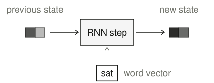
The simplest version, often called an Elman network, computes the new state with one layer:

$$\mathbf{h}_t = \tanh(\mathbf{W}\mathbf{x}_t + \mathbf{U}\mathbf{h}_{t-1} + \mathbf{b})$$

The matrix $\mathbf{W}$ weighs the new word, $\mathbf{U}$ weighs the previous state, and $\mathbf{b}$ is a bias. The hyperbolic tangent, $\tanh$, squashes each number of the sum into the range from $-1$ to $1$. Before the first word the state is all zeros, $\mathbf{h}_0 = \mathbf{0}$.

Elman's 1990 network had this structure. It copied the hidden layer at each step into a set of "context units", which fed back into the hidden layer together with the next input [3]. An earlier network by Michael Jordan, which Elman built on, had fed back its outputs instead. Because the hidden layer is trained, what it carries forward is learned too.

Working through "we sat"

To follow the arithmetic, we can give every vector two numbers. Take these weights, with $\mathbf{b} = \mathbf{0}$:

$$\mathbf{W} = \begin{pmatrix} 0.5 & 1 \\ 1 & -0.5 \end{pmatrix}, \qquad \mathbf{U} = \begin{pmatrix} 1 & -0.5 \\ 0.5 & 1 \end{pmatrix}$$

and these embeddings for the first two words, written as rows to save space:

At the first step the previous state is zero, so only the word contributes:

$${\mathbf{h}_1 = \tanh(\mathbf{W}\mathbf{x}_{\text{we}})} = {\tanh(0.5,\ -0.5)} = (0.46,\ -0.46)$$

At the second step the new word and the previous state both enter the sum:

$${\mathbf{W}\mathbf{x}_{\text{sat}} + \mathbf{U}\mathbf{h}_1} = {(0.50,\ 0.50) + (0.69,\ -0.23)} = (1.19,\ 0.27)$$ $$\mathbf{h}_2 = \tanh(1.19,\ 0.27) = (0.83,\ 0.26)$$

The state $\mathbf{h}_2$ depends on "sat" through $\mathbf{W}\mathbf{x}_{\text{sat}}$ and on "we" through $\mathbf{U}\mathbf{h}_1$. Had the sentence started with a different word, $\mathbf{h}_1$ would differ and so would $\mathbf{h}_2$.

The same weights at every step

Each later word goes through the same computation with the same $\mathbf{W}$, $\mathbf{U}$ and $\mathbf{b}$. Drawn out over the whole sentence, the RNN becomes a chain of identical steps, called the unrolled network:

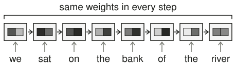
The shading shows the two numbers of each state, from $-1$ (light) to $1$ (dark). If we write one step as a function $f$, so that $\mathbf{h}_t = f(\mathbf{x}_t, \mathbf{h}_{t-1})$, then unrolling three steps gives

$$\mathbf{h}_3 = f(\mathbf{x}_3,\ f(\mathbf{x}_2,\ f(\mathbf{x}_1,\ \mathbf{h}_0)))$$

so the state after any word depends on every word before it [4]. The state $\mathbf{h}_8$ after "river" is a function of all eight words.

Sharing the weights also fixes the size of the model. With word embeddings of $d$ numbers and a state of $k$ numbers, $\mathbf{W}$ holds $k \times d$ weights, $\mathbf{U}$ holds $k \times k$ and $\mathbf{b}$ holds $k$, whatever the length of the sentence. With $d = k = 100$, that is $20{,}100$ numbers, for a sentence of eight words or eighty.

What the state encodes is learned from the task. Elman trained a network with 150 hidden units to predict the next word in a stream of 27,354 words from 10,000 short generated sentences, with every word given as a code that said nothing about its meaning. When he averaged the hidden states for each of the 29 words and clustered them, nouns and verbs separated, and the nouns split into animate and inanimate, then into humans, animals, foods and breakable objects [3]. The network had found these classes from word order alone.

Acceptors and encoders read the final state

Once the chain has read the sentence, there are several ways to take an answer from it. The simplest uses only the last state. An RNN used this way is an acceptor: it reads the whole sequence and makes one prediction from $\mathbf{h}_8$, for example the topic or the sentiment of the sentence, and the loss is computed from that single prediction [4]. The name comes from finite-state acceptors, which read a string to the end and then accept or reject it.

An encoder also keeps only the final state but doesn't make a decision from it. It hands $\mathbf{h}_8$ to another model as a fixed-size vector standing for the whole sentence, to be combined with other information there.

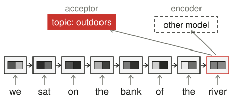
Either way, a sentence of any length becomes a vector of $k$ numbers, which a feed-forward classifier can take as input.

Transducers read every state

A transducer makes a prediction from the state after every word, so it produces one output per input. Part-of-speech tagging works this way. Each word gets a tag such as PRON for a pronoun, DET for a determiner such as "the", or ADP for a preposition such as "on" or "of":

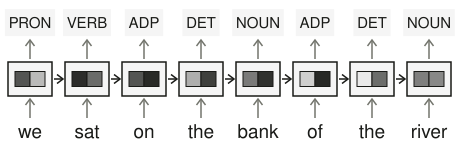
The tag for "bank" is predicted from $\mathbf{h}_5$, which depends on "we sat on the bank". In a hidden Markov model tagger, by contrast, the probability of each tag depends only on the tag before it. Training a transducer computes a loss at every step and adds the losses up [4].

A language model without the Markov assumption

A language model is a transducer whose output at step $t$ is a guess at word $t+1$:

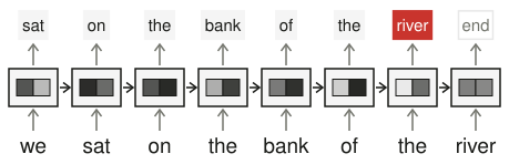
An output matrix $\mathbf{V}$ with one row per vocabulary word turns the state into one score per word, and softmax turns the scores into probabilities:

$$\mathbf{y}_t = \mathbf{V}\mathbf{h}_t$$ $${P(w_{t+1} = i \mid w_1, \dots, w_t)} = \frac{e^{y_{t,i}}}{\sum_j e^{y_{t,j}}}$$

Since $\mathbf{h}_t$ depends on every word so far, the context of each prediction is the whole sentence up to that point. Nothing is cut off, so the probability of a sentence is the exact chain-rule product, with no Markov approximation:

$${P(w_1, \dots, w_n)} = \prod_{t=1}^{n} {P(w_t \mid w_1, \dots, w_{t-1})}$$

We can follow one prediction in our two-number network. Continuing the computation through "we sat on the bank of the" gives $\mathbf{h}_7 = (-0.90,\ 0.24)$. To see the arithmetic, we shrink the vocabulary to four words. The row of $\mathbf{V}$ for "river" is $(-1.0,\ 0)$, so its score is $(-1.0)(-0.90) + 0 \cdot 0.24 = 0.90$. The rows for "lake", "road" and "sat", $(-0.5,\ 0.5)$, $(0.5,\ 0)$ and $(0.5,\ -0.5)$, give scores of $0.57$, $-0.45$ and $-0.57$. Softmax turns the four scores into river $0.453$, lake $0.326$, road $0.117$ and sat $0.104$.

In 2010, Mikolov and colleagues used this kind of simple recurrent network as the language model of a speech recognizer, with a sigmoid in place of $\tanh$ and between 30 and 500 hidden units [2]. They measured perplexity, the geometric mean of $1/P(w \mid c)$ over the words of held-out text, where lower means better predictions. Trained on 6.4 million words of newspaper text, a single RNN reached a perplexity of 171, against 221 for a 5-gram model trained on the same words. A mix of three RNNs and the 5-gram model, with the RNNs still updating as they read the test data, cut the recognizer's word error rate from 13.5% to 11.1%, about 18% fewer errors. The cost was training time: the largest models took several weeks to train.

How is a loop trained?

Training should raise the probability of each correct next word. For the step that predicts "river", the loss is

$$L_7 = -\log 0.453 \approx 0.79$$

and the loss for the sentence adds one such term per step:

$$L = \sum_{t=1}^{n-1} -\log {P(w_{t+1} \mid w_1, \dots, w_t)}$$

In a feed-forward network each weight belongs to one layer, and its effect on the loss passes through the layers above it once. Here $L_7$ depends on $\mathbf{W}$ at all seven steps behind "river" and on $\mathbf{U}$ at every step after the first: $\mathbf{U}$ shapes $\mathbf{h}_2$, which feeds into $\mathbf{h}_3$, and so on up to $\mathbf{h}_7$, and it acts again at each of those steps. The chain of uses grows with every word in the sentence. To adjust either matrix, the error at "river" has to be traced back through a loop that ran seven times.

References

1. Bengio, Y., et al. (2003). A neural probabilistic language model. Journal of Machine Learning Research 3. jmlr.org ↩
2. Mikolov, T., et al. (2010). Recurrent neural network based language model. Proceedings of Interspeech 2010. doi:10.21437/Interspeech.2010-343 ↩
3. Elman, J. L. (1990). Finding structure in time. Cognitive Science 14(2). doi:10.1207/s15516709cog1402_1 ↩
4. Goldberg, Y. (2016). A primer on neural network models for natural language processing. Journal of Artificial Intelligence Research 57. doi:10.1613/jair.4992 ↩